We will define in a very simple way each one of the basic concepts used in a quality control system by variables applied in the inspection of packaging.

Before we will define what we understand by variables.

WHAT TYPES OF VARIABLES DO WE KNOW?

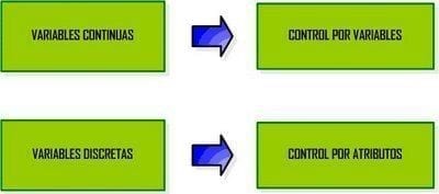
There are two types of variables to consider, Continuous Variables and Discrete Variables

Continuous variables
The continuous variables are those that are measured.
Discrete variables
the discrete variables are counted.
The former give rise to control by variables and the latter control by attributes.

The quality characteristics that we will call variables are all those that can be represented by a number. For example, the measurement of a bolt, the resistance of wire resistors, the content of ashes in coal, etc., etc.
Attributes are those quality characteristics that can not be measured, whose general dimension can not be represented by a figure. As for example we can take the visual imperfections of the surfaces of the products, such as spots, differences of tone, aspects of a welding, etc., etc.
Finally, we must bear in mind that both the processes and the finished lots can be inspected by attributes or by variables.

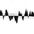
The best way is to serve as a practical example. Suppose we are controlling the length of the flange of the body of the container. After a series of measurements, we make a graph with them as shown in figure 1. We have on the abscissa axis the found values ​​of the flange lengths and in ordinate the number of packages.

With this graph in view we will define as:

Variable : The parameter to measure. In this case the flange length.

Frequency : Number of times a variable is repeated. In our example the number of containers.

Route: Range in which a variable moves. Between 2.1 and 2.8 mm (Tab length values)

Interval : Grouping of values ​​of a variable within a certain distance. For example: Grouping of all values ​​between 2.3 and 2.4 in the value 2.4.

Amplitude : Difference between extreme values ​​of the route. In our example of the tabs: 2.8 – 2.1 = 0.7 of amplitude.

Average: (or arithmetic mean): Sum of all values ​​divided by the total number of data

X = (10*2.1 + 20*2.3 + 30*2.4 + 40*2.5 + 50*2.6 + 40*2.7 + 30*2.8) / (10 + 20 + 30 + 40 + 50 + 40 + 30 )  =  ( 21 + 46 + 72 + 100 + 130 + 108 + 84) / 220 = 2.55

Median: Value of the distribution, supposedly ordered from least to greatest, leaving to its left and right the same number of frequencies, that is, the value that occupies the central place, assuming an odd number of data. If the number of data were even, it can be said that there are two medium values ​​and the arithmetic mean is taken between them.

Following the previous example of the tab length we would have:

Frequencies = 10 + 20 + 30 + 40 + 50 + 40 + 30 = 220

220                       would be the absolute or cumulative frequency

Frequency center = 220/2 = 110

Therefore, the median would be : 2.6 , since this is the value of the variable that occupies the 110th place starting from the beginning.

Frequency Cumulative frequency Variable (m / m )

10 10 2.1

20 30 2.3

30 60 2.4

40 100 2,5

50 150 2.6

40 190 2.7

30 220 2.8

More information in:

http://html.rincondelvago.com/control-de-calidad-estadistico.html

http://gdcalidad.blogspot.com/2009/04/graficos-de-control-por-variables.html